Spam_mail
스팸 메일 분류로 배우는 머신러닝 Using R
안녕하세요. 이번 글에서는 권재명선생님께서 쓰신 책의 주제와 코드를 중심으로
의사결정나무(Decision Tree)와 앙상블(Ensemble) 기법 중 하나인 랜덤포레스트(Random Forest)를 활용하여
스팸 메일을 분류하는 모델을 학습시켜 보도록 하겠습니다.
우선 데이터는 CUI Machine Learning Reapository에서 ‘spambase.data’, ‘spambase.names’ 파일을
setwd로 설정한 디렉토리에 다운받아 저장합니다.
reference: Dua, D. and Graff, C. (2019). UCI Machine Learning Repository [http://archive.ics.uci.edu/ml]. Irvine, CA: University of California, School of Information and Computer Science.
해당 데이터에 대한 자세한 설명은 링크를 참고해주세요.
요약하자면,
-
행: 4,601(사례), 열: 58(변수/Feature)
-
58번째 Feature는
Label Data로 스팸인 지(spam=1) 아닌지(=0)를 나타냄
연구 절차는 다음과 같습니다.
- 시스템 세팅
- 데이터 이해(기초 분석 및 시각화)
- 데이터 분할
- 의사결정나무 모형(Decision Tree)
- 랜덤포레스트(Random Forest)
- 모형 평가, 해석 및 선택
시스템 세팅
먼저 관련 패키지를 설치하고, 불러옵니다.
#install.packages(c( "randomForest", "rpart","boot","data.table", caret" ))
#install.packages(c( "rattle", "rpart.plot", "RColorBrewer", "e1071"))

library(dplyr); library(ggplot2); library(MASS); library(randomForest); library(rpart); library(boot); library(data.table); library(caret)
##
## Attaching package: 'dplyr'

## The following objects are masked from 'package:stats':
##
##     filter, lag

## The following objects are masked from 'package:base':
##
##     intersect, setdiff, setequal, union

##
## Attaching package: 'MASS'

## The following object is masked from 'package:dplyr':
##
##     select

## randomForest 4.6-14

## Type rfNews() to see new features/changes/bug fixes.

##
## Attaching package: 'randomForest'

## The following object is masked from 'package:ggplot2':
##
##     margin

## The following object is masked from 'package:dplyr':
##
##     combine

##
## Attaching package: 'data.table'

## The following objects are masked from 'package:dplyr':
##
##     between, first, last

## Loading required package: lattice

##
## Attaching package: 'lattice'

## The following object is masked from 'package:boot':
##
##     melanoma
다음으로는 데이터를 로드합니다.
data <- tbl_df(read.table("spambase.data", strip.white = TRUE,
                          sep=",", header = FALSE)) #dplyr 패키지 함수 입니다.
                                                    #해당 파일이 워크디렉토리안에 저장되어 있어야 합니다.
names(data) <- #Feature의 이름을 입력합니다.
  c('word_freq_make', 'word_freq_address', 'word_freq_all', 'word_freq_3d', 'word_freq_our',
    'word_freq_over', 'word_freq_remove', 'word_freq_internet', 'word_freq_order', 'word_freq_mail',
    'word_freq_receive', 'word_freq_will', 'word_freq_people', 'word_freq_report', 'word_freq_addresses',
    'word_freq_free', 'word_freq_business', 'word_freq_email', 'word_freq_you', 'word_freq_credit',
    'word_freq_your', 'word_freq_font', 'word_freq_000', 'word_freq_money', 'word_freq_hp',
    'word_freq_hpl', 'word_freq_george', 'word_freq_650', 'word_freq_lab', 'word_freq_labs',
    'word_freq_telnet', 'word_freq_857', 'word_freq_data', 'word_freq_415', 'word_freq_85',
    'word_freq_technology', 'word_freq_1999', 'word_freq_parts', 'word_freq_pm', 'word_freq_direct',
    'word_freq_cs', 'word_freq_meeting', 'word_freq_original', 'word_freq_project', 'word_freq_re',
    'word_freq_edu', 'word_freq_table', 'word_freq_conference', 'char_freq_;', 'char_freq_(',
    'char_freq_[', 'char_freq_!', 'char_freq_$', 'char_freq_#', 'capital_run_length_average',
    'capital_run_length_longest', 'capital_run_length_total', 'class' #class 변수가 Label Data 입니다.
  )

data$class <- factor(data$class) #범주형 변수로 변환(스팸메일 인지/아닌지 이기 때문에 범주형 입니다.)
데이터 이해(기초 분석 및 시각화)
간단한 코드를 통해 데이터에 대한 이해를 높일 수 있습니다.
데이터의 내용을 이해하지 못하면, 머신러닝 모델 결과의 올바른 해석이 불가능합니다.
또한 상관 계수와 산점도를 확인해 보는 것도 데이터의 이해를 높이는데 좋은 방법입니다.
glimpse(data) #str(data) 비교해보는 것도 좋을 것 같습니다.
## Observations: 4,601
## Variables: 58
## $ word_freq_make             <dbl> 0.00, 0.21, 0.06, 0.00, 0.00, 0.00, 0.00...
## $ word_freq_address          <dbl> 0.64, 0.28, 0.00, 0.00, 0.00, 0.00, 0.00...
## $ word_freq_all              <dbl> 0.64, 0.50, 0.71, 0.00, 0.00, 0.00, 0.00...
## $ word_freq_3d               <dbl> 0, 0, 0, 0, 0, 0, 0, 0, 0, 0, 0, 0, 0, 0...
## $ word_freq_our              <dbl> 0.32, 0.14, 1.23, 0.63, 0.63, 1.85, 1.92...
## $ word_freq_over             <dbl> 0.00, 0.28, 0.19, 0.00, 0.00, 0.00, 0.00...
## $ word_freq_remove           <dbl> 0.00, 0.21, 0.19, 0.31, 0.31, 0.00, 0.00...
## $ word_freq_internet         <dbl> 0.00, 0.07, 0.12, 0.63, 0.63, 1.85, 0.00...
## $ word_freq_order            <dbl> 0.00, 0.00, 0.64, 0.31, 0.31, 0.00, 0.00...
## $ word_freq_mail             <dbl> 0.00, 0.94, 0.25, 0.63, 0.63, 0.00, 0.64...
## $ word_freq_receive          <dbl> 0.00, 0.21, 0.38, 0.31, 0.31, 0.00, 0.96...
## $ word_freq_will             <dbl> 0.64, 0.79, 0.45, 0.31, 0.31, 0.00, 1.28...
## $ word_freq_people           <dbl> 0.00, 0.65, 0.12, 0.31, 0.31, 0.00, 0.00...
## $ word_freq_report           <dbl> 0.00, 0.21, 0.00, 0.00, 0.00, 0.00, 0.00...
## $ word_freq_addresses        <dbl> 0.00, 0.14, 1.75, 0.00, 0.00, 0.00, 0.00...
## $ word_freq_free             <dbl> 0.32, 0.14, 0.06, 0.31, 0.31, 0.00, 0.96...
## $ word_freq_business         <dbl> 0.00, 0.07, 0.06, 0.00, 0.00, 0.00, 0.00...
## $ word_freq_email            <dbl> 1.29, 0.28, 1.03, 0.00, 0.00, 0.00, 0.32...
## $ word_freq_you              <dbl> 1.93, 3.47, 1.36, 3.18, 3.18, 0.00, 3.85...
## $ word_freq_credit           <dbl> 0.00, 0.00, 0.32, 0.00, 0.00, 0.00, 0.00...
## $ word_freq_your             <dbl> 0.96, 1.59, 0.51, 0.31, 0.31, 0.00, 0.64...
## $ word_freq_font             <dbl> 0, 0, 0, 0, 0, 0, 0, 0, 0, 0, 0, 0, 0, 0...
## $ word_freq_000              <dbl> 0.00, 0.43, 1.16, 0.00, 0.00, 0.00, 0.00...
## $ word_freq_money            <dbl> 0.00, 0.43, 0.06, 0.00, 0.00, 0.00, 0.00...
## $ word_freq_hp               <dbl> 0, 0, 0, 0, 0, 0, 0, 0, 0, 0, 0, 0, 0, 0...
## $ word_freq_hpl              <dbl> 0, 0, 0, 0, 0, 0, 0, 0, 0, 0, 0, 0, 0, 0...
## $ word_freq_george           <dbl> 0, 0, 0, 0, 0, 0, 0, 0, 0, 0, 0, 0, 0, 0...
## $ word_freq_650              <dbl> 0.00, 0.00, 0.00, 0.00, 0.00, 0.00, 0.00...
## $ word_freq_lab              <dbl> 0, 0, 0, 0, 0, 0, 0, 0, 0, 0, 0, 0, 0, 0...
## $ word_freq_labs             <dbl> 0, 0, 0, 0, 0, 0, 0, 0, 0, 0, 0, 0, 0, 0...
## $ word_freq_telnet           <dbl> 0, 0, 0, 0, 0, 0, 0, 0, 0, 0, 0, 0, 0, 0...
## $ word_freq_857              <dbl> 0, 0, 0, 0, 0, 0, 0, 0, 0, 0, 0, 0, 0, 0...
## $ word_freq_data             <dbl> 0.00, 0.00, 0.00, 0.00, 0.00, 0.00, 0.00...
## $ word_freq_415              <dbl> 0, 0, 0, 0, 0, 0, 0, 0, 0, 0, 0, 0, 0, 0...
## $ word_freq_85               <dbl> 0, 0, 0, 0, 0, 0, 0, 0, 0, 0, 0, 0, 0, 0...
## $ word_freq_technology       <dbl> 0.00, 0.00, 0.00, 0.00, 0.00, 0.00, 0.00...
## $ word_freq_1999             <dbl> 0.00, 0.07, 0.00, 0.00, 0.00, 0.00, 0.00...
## $ word_freq_parts            <dbl> 0, 0, 0, 0, 0, 0, 0, 0, 0, 0, 0, 0, 0, 0...
## $ word_freq_pm               <dbl> 0, 0, 0, 0, 0, 0, 0, 0, 0, 0, 0, 0, 0, 0...
## $ word_freq_direct           <dbl> 0.00, 0.00, 0.06, 0.00, 0.00, 0.00, 0.00...
## $ word_freq_cs               <dbl> 0, 0, 0, 0, 0, 0, 0, 0, 0, 0, 0, 0, 0, 0...
## $ word_freq_meeting          <dbl> 0, 0, 0, 0, 0, 0, 0, 0, 0, 0, 0, 0, 0, 0...
## $ word_freq_original         <dbl> 0.00, 0.00, 0.12, 0.00, 0.00, 0.00, 0.00...
## $ word_freq_project          <dbl> 0.00, 0.00, 0.00, 0.00, 0.00, 0.00, 0.00...
## $ word_freq_re               <dbl> 0.00, 0.00, 0.06, 0.00, 0.00, 0.00, 0.00...
## $ word_freq_edu              <dbl> 0.00, 0.00, 0.06, 0.00, 0.00, 0.00, 0.00...
## $ word_freq_table            <dbl> 0, 0, 0, 0, 0, 0, 0, 0, 0, 0, 0, 0, 0, 0...
## $ word_freq_conference       <dbl> 0, 0, 0, 0, 0, 0, 0, 0, 0, 0, 0, 0, 0, 0...
## $ `char_freq_;`              <dbl> 0.000, 0.000, 0.010, 0.000, 0.000, 0.000...
## $ `char_freq_(`              <dbl> 0.000, 0.132, 0.143, 0.137, 0.135, 0.223...
## $ `char_freq_[`              <dbl> 0.000, 0.000, 0.000, 0.000, 0.000, 0.000...
## $ `char_freq_!`              <dbl> 0.778, 0.372, 0.276, 0.137, 0.135, 0.000...
## $ `char_freq_$`              <dbl> 0.000, 0.180, 0.184, 0.000, 0.000, 0.000...
## $ `char_freq_#`              <dbl> 0.000, 0.048, 0.010, 0.000, 0.000, 0.000...
## $ capital_run_length_average <dbl> 3.756, 5.114, 9.821, 3.537, 3.537, 3.000...
## $ capital_run_length_longest <int> 61, 101, 485, 40, 40, 15, 4, 11, 445, 43...
## $ capital_run_length_total   <int> 278, 1028, 2259, 191, 191, 54, 112, 49, ...
## $ class                      <fct> 1, 1, 1, 1, 1, 1, 1, 1, 1, 1, 1, 1, 1, 1...
summary(data)
##  word_freq_make   word_freq_address word_freq_all     word_freq_3d
##  Min.   :0.0000   Min.   : 0.000    Min.   :0.0000   Min.   : 0.00000
##  1st Qu.:0.0000   1st Qu.: 0.000    1st Qu.:0.0000   1st Qu.: 0.00000
##  Median :0.0000   Median : 0.000    Median :0.0000   Median : 0.00000
##  Mean   :0.1046   Mean   : 0.213    Mean   :0.2807   Mean   : 0.06542
##  3rd Qu.:0.0000   3rd Qu.: 0.000    3rd Qu.:0.4200   3rd Qu.: 0.00000
##  Max.   :4.5400   Max.   :14.280    Max.   :5.1000   Max.   :42.81000
##  word_freq_our     word_freq_over   word_freq_remove word_freq_internet
##  Min.   : 0.0000   Min.   :0.0000   Min.   :0.0000   Min.   : 0.0000
##  1st Qu.: 0.0000   1st Qu.:0.0000   1st Qu.:0.0000   1st Qu.: 0.0000
##  Median : 0.0000   Median :0.0000   Median :0.0000   Median : 0.0000
##  Mean   : 0.3122   Mean   :0.0959   Mean   :0.1142   Mean   : 0.1053
##  3rd Qu.: 0.3800   3rd Qu.:0.0000   3rd Qu.:0.0000   3rd Qu.: 0.0000
##  Max.   :10.0000   Max.   :5.8800   Max.   :7.2700   Max.   :11.1100
##  word_freq_order   word_freq_mail    word_freq_receive word_freq_will
##  Min.   :0.00000   Min.   : 0.0000   Min.   :0.00000   Min.   :0.0000
##  1st Qu.:0.00000   1st Qu.: 0.0000   1st Qu.:0.00000   1st Qu.:0.0000
##  Median :0.00000   Median : 0.0000   Median :0.00000   Median :0.1000
##  Mean   :0.09007   Mean   : 0.2394   Mean   :0.05982   Mean   :0.5417
##  3rd Qu.:0.00000   3rd Qu.: 0.1600   3rd Qu.:0.00000   3rd Qu.:0.8000
##  Max.   :5.26000   Max.   :18.1800   Max.   :2.61000   Max.   :9.6700
##  word_freq_people  word_freq_report   word_freq_addresses word_freq_free
##  Min.   :0.00000   Min.   : 0.00000   Min.   :0.0000      Min.   : 0.0000
##  1st Qu.:0.00000   1st Qu.: 0.00000   1st Qu.:0.0000      1st Qu.: 0.0000
##  Median :0.00000   Median : 0.00000   Median :0.0000      Median : 0.0000
##  Mean   :0.09393   Mean   : 0.05863   Mean   :0.0492      Mean   : 0.2488
##  3rd Qu.:0.00000   3rd Qu.: 0.00000   3rd Qu.:0.0000      3rd Qu.: 0.1000
##  Max.   :5.55000   Max.   :10.00000   Max.   :4.4100      Max.   :20.0000
##  word_freq_business word_freq_email  word_freq_you    word_freq_credit
##  Min.   :0.0000     Min.   :0.0000   Min.   : 0.000   Min.   : 0.00000
##  1st Qu.:0.0000     1st Qu.:0.0000   1st Qu.: 0.000   1st Qu.: 0.00000
##  Median :0.0000     Median :0.0000   Median : 1.310   Median : 0.00000
##  Mean   :0.1426     Mean   :0.1847   Mean   : 1.662   Mean   : 0.08558
##  3rd Qu.:0.0000     3rd Qu.:0.0000   3rd Qu.: 2.640   3rd Qu.: 0.00000
##  Max.   :7.1400     Max.   :9.0900   Max.   :18.750   Max.   :18.18000
##  word_freq_your    word_freq_font    word_freq_000    word_freq_money
##  Min.   : 0.0000   Min.   : 0.0000   Min.   :0.0000   Min.   : 0.00000
##  1st Qu.: 0.0000   1st Qu.: 0.0000   1st Qu.:0.0000   1st Qu.: 0.00000
##  Median : 0.2200   Median : 0.0000   Median :0.0000   Median : 0.00000
##  Mean   : 0.8098   Mean   : 0.1212   Mean   :0.1016   Mean   : 0.09427
##  3rd Qu.: 1.2700   3rd Qu.: 0.0000   3rd Qu.:0.0000   3rd Qu.: 0.00000
##  Max.   :11.1100   Max.   :17.1000   Max.   :5.4500   Max.   :12.50000
##   word_freq_hp     word_freq_hpl     word_freq_george  word_freq_650
##  Min.   : 0.0000   Min.   : 0.0000   Min.   : 0.0000   Min.   :0.0000
##  1st Qu.: 0.0000   1st Qu.: 0.0000   1st Qu.: 0.0000   1st Qu.:0.0000
##  Median : 0.0000   Median : 0.0000   Median : 0.0000   Median :0.0000
##  Mean   : 0.5495   Mean   : 0.2654   Mean   : 0.7673   Mean   :0.1248
##  3rd Qu.: 0.0000   3rd Qu.: 0.0000   3rd Qu.: 0.0000   3rd Qu.:0.0000
##  Max.   :20.8300   Max.   :16.6600   Max.   :33.3300   Max.   :9.0900
##  word_freq_lab      word_freq_labs   word_freq_telnet   word_freq_857
##  Min.   : 0.00000   Min.   :0.0000   Min.   : 0.00000   Min.   :0.00000
##  1st Qu.: 0.00000   1st Qu.:0.0000   1st Qu.: 0.00000   1st Qu.:0.00000
##  Median : 0.00000   Median :0.0000   Median : 0.00000   Median :0.00000
##  Mean   : 0.09892   Mean   :0.1029   Mean   : 0.06475   Mean   :0.04705
##  3rd Qu.: 0.00000   3rd Qu.:0.0000   3rd Qu.: 0.00000   3rd Qu.:0.00000
##  Max.   :14.28000   Max.   :5.8800   Max.   :12.50000   Max.   :4.76000
##  word_freq_data     word_freq_415      word_freq_85     word_freq_technology
##  Min.   : 0.00000   Min.   :0.00000   Min.   : 0.0000   Min.   :0.00000
##  1st Qu.: 0.00000   1st Qu.:0.00000   1st Qu.: 0.0000   1st Qu.:0.00000
##  Median : 0.00000   Median :0.00000   Median : 0.0000   Median :0.00000
##  Mean   : 0.09723   Mean   :0.04784   Mean   : 0.1054   Mean   :0.09748
##  3rd Qu.: 0.00000   3rd Qu.:0.00000   3rd Qu.: 0.0000   3rd Qu.:0.00000
##  Max.   :18.18000   Max.   :4.76000   Max.   :20.0000   Max.   :7.69000
##  word_freq_1999  word_freq_parts   word_freq_pm      word_freq_direct
##  Min.   :0.000   Min.   :0.0000   Min.   : 0.00000   Min.   :0.00000
##  1st Qu.:0.000   1st Qu.:0.0000   1st Qu.: 0.00000   1st Qu.:0.00000
##  Median :0.000   Median :0.0000   Median : 0.00000   Median :0.00000
##  Mean   :0.137   Mean   :0.0132   Mean   : 0.07863   Mean   :0.06483
##  3rd Qu.:0.000   3rd Qu.:0.0000   3rd Qu.: 0.00000   3rd Qu.:0.00000
##  Max.   :6.890   Max.   :8.3300   Max.   :11.11000   Max.   :4.76000
##   word_freq_cs     word_freq_meeting word_freq_original word_freq_project
##  Min.   :0.00000   Min.   : 0.0000   Min.   :0.0000     Min.   : 0.0000
##  1st Qu.:0.00000   1st Qu.: 0.0000   1st Qu.:0.0000     1st Qu.: 0.0000
##  Median :0.00000   Median : 0.0000   Median :0.0000     Median : 0.0000
##  Mean   :0.04367   Mean   : 0.1323   Mean   :0.0461     Mean   : 0.0792
##  3rd Qu.:0.00000   3rd Qu.: 0.0000   3rd Qu.:0.0000     3rd Qu.: 0.0000
##  Max.   :7.14000   Max.   :14.2800   Max.   :3.5700     Max.   :20.0000
##   word_freq_re     word_freq_edu     word_freq_table    word_freq_conference
##  Min.   : 0.0000   Min.   : 0.0000   Min.   :0.000000   Min.   : 0.00000
##  1st Qu.: 0.0000   1st Qu.: 0.0000   1st Qu.:0.000000   1st Qu.: 0.00000
##  Median : 0.0000   Median : 0.0000   Median :0.000000   Median : 0.00000
##  Mean   : 0.3012   Mean   : 0.1798   Mean   :0.005444   Mean   : 0.03187
##  3rd Qu.: 0.1100   3rd Qu.: 0.0000   3rd Qu.:0.000000   3rd Qu.: 0.00000
##  Max.   :21.4200   Max.   :22.0500   Max.   :2.170000   Max.   :10.00000
##   char_freq_;       char_freq_(     char_freq_[       char_freq_!
##  Min.   :0.00000   Min.   :0.000   Min.   :0.00000   Min.   : 0.0000
##  1st Qu.:0.00000   1st Qu.:0.000   1st Qu.:0.00000   1st Qu.: 0.0000
##  Median :0.00000   Median :0.065   Median :0.00000   Median : 0.0000
##  Mean   :0.03857   Mean   :0.139   Mean   :0.01698   Mean   : 0.2691
##  3rd Qu.:0.00000   3rd Qu.:0.188   3rd Qu.:0.00000   3rd Qu.: 0.3150
##  Max.   :4.38500   Max.   :9.752   Max.   :4.08100   Max.   :32.4780
##   char_freq_$       char_freq_#       capital_run_length_average
##  Min.   :0.00000   Min.   : 0.00000   Min.   :   1.000
##  1st Qu.:0.00000   1st Qu.: 0.00000   1st Qu.:   1.588
##  Median :0.00000   Median : 0.00000   Median :   2.276
##  Mean   :0.07581   Mean   : 0.04424   Mean   :   5.191
##  3rd Qu.:0.05200   3rd Qu.: 0.00000   3rd Qu.:   3.706
##  Max.   :6.00300   Max.   :19.82900   Max.   :1102.500
##  capital_run_length_longest capital_run_length_total class
##  Min.   :   1.00            Min.   :    1.0          0:2788
##  1st Qu.:   6.00            1st Qu.:   35.0          1:1813
##  Median :  15.00            Median :   95.0
##  Mean   :  52.17            Mean   :  283.3
##  3rd Qu.:  43.00            3rd Qu.:  266.0
##  Max.   :9989.00            Max.   :15841.0
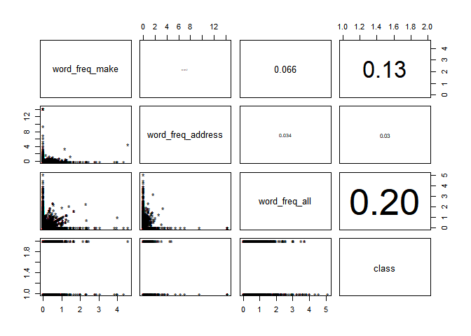
data_1 <- subset(data, select = c(word_freq_make, word_freq_address, word_freq_all, class))
#모든 변수를 한꺼번에 그리는 것이 쉽지 않아, 부분적으로 먼저 확인해보겠습니다.

#아래 코드는 산점도 행렬의 위쪽에 상관계수 숫자를 집어넣는 사용자 정의 함수 입니다.
#출처: https://rfriend.tistory.com/83 [R, Python 분석과 프로그래밍의 친구 (by R Friend)]

panel.cor <- function(x, y, digits = 2, prefix = "", cex.cor, ...)
{
  usr <- par("usr"); on.exit(par(usr))
  par(usr = c(0, 1, 0, 1))
  r <- abs(cor(x, y))
  txt <- format(c(r, 0.123456789), digits = digits)[1]
  txt <- paste0(prefix, txt)
  if(missing(cex.cor)) cex.cor <- 0.8/strwidth(txt)
  text(0.5, 0.5, txt, cex = cex.cor * r * 5)
}

pairs(data_1,
      upper.panel = panel.cor, # 위쪽에는 상관계수 비례)
      pch="*"
      )
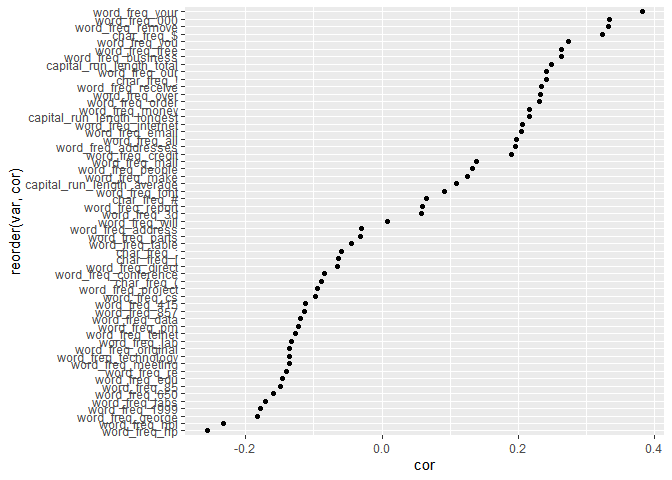
#57개 Feature 중 Label Data의 Class와 상관 관계가 가장 높은 변수는 어떤 변수인지 살펴보겠습니다.
tmp <- as.data.frame(cor(data[,-58], as.numeric(data$class)))
tmp <- tmp %>% rename(cor=V1)
tmp$var <- rownames(tmp)
tmp %>%
  ggplot(aes(reorder(var, cor), cor)) +
  geom_point() +
  coord_flip()
데이터 분할
데이터 분할에 앞서서 데이터 전처리 과정이 필요합니다.
본 데이터는 CUI Machine Learning Reapository에서 전처리가 되어 제공되는 데이터지만,
본 연구에서 적용하는 RandomForest 패키지에서는 특수문자가 포함된 Feature는 모델에 사용할 수 없습니다.권재명(2017)
따라서, make.names함수를 활용하여 이 문제를 해결합니다.
old_names <- names(data)
new_names <- make.names(names(data), unique = TRUE)
cbind(old_names, new_names) [old_names!=new_names, ]
##      old_names     new_names
## [1,] "char_freq_;" "char_freq_."
## [2,] "char_freq_(" "char_freq_..1"
## [3,] "char_freq_[" "char_freq_..2"
## [4,] "char_freq_!" "char_freq_..3"
## [5,] "char_freq_$" "char_freq_..4"
## [6,] "char_freq_#" "char_freq_..5"
names(data) <- new_names
다음으로 caret패키지를 활용하여 데이터를 분할합니다.
여러가지 데이터 분할 방법이 있지만, 저는 이 방법이 가장 편하고 익숙합니다.^^
intrain<-createDataPartition(y=data$class, p=0.7, list=FALSE)
train<-data[intrain, ] #학습용 데이터 셋
test<-data[-intrain, ] #평가용 데이터 셋
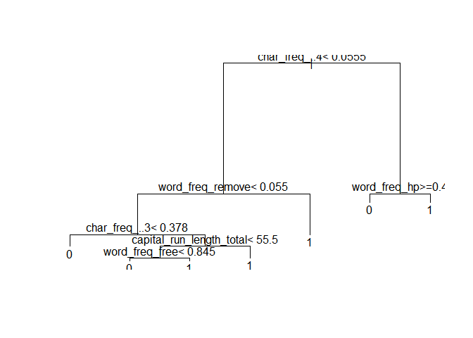
Decision Tree
일반적으로 트리를 생성할 때 R에서는 tree, rpart, party와 같은 패키지를 많이 활용합니다.
하지만, 강력한 시각화를 장점으로 하고 있는 R에서 유독 Decision Tree만 시각화를 하면 괜히 미안해집니다.
이를 위해 DODOMIRA님께서 제시하신 rattle 패키지의 fancyrpartplot 함수를 활용한 방법으로 트리를 플로팅하였습니다.
트리 해석 또한 해당 블로그를 참고하시면 될 것 같습니다.
#install.packages(c("rattle", "rpart.plot", "RColorBrewer"))
library(rattle)                 # Fancy tree plot
## Rattle: A free graphical interface for data science with R.
## Version 5.3.0 Copyright (c) 2006-2018 Togaware Pty Ltd.
## Type 'rattle()' to shake, rattle, and roll your data.

##
## Attaching package: 'rattle'

## The following object is masked from 'package:randomForest':
##
##     importance
library(rpart.plot)           # Enhanced tree plots
library(RColorBrewer)           # Color selection for fancy tree
rpart_spam<-rpart(class~. , data=data, method="class")
plot(rpart_spam); text(rpart_spam)      #원래 rpart 패키지 트리
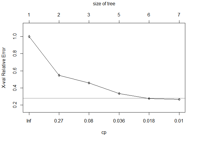
printcp(rpart_spam); plotcp(rpart_spam) #과적합 방지를 위해 cp(Complexity Parameter, 복잡성 매개변수)값을 통해 가지치기 실시
##
## Classification tree:
## rpart(formula = class ~ ., data = data, method = "class")
##
## Variables actually used in tree construction:
## [1] capital_run_length_total char_freq_..3            char_freq_..4
## [4] word_freq_free           word_freq_hp             word_freq_remove
##
## Root node error: 1813/4601 = 0.39404
##
## n= 4601
##
##         CP nsplit rel error  xerror     xstd
## 1 0.476558      0   1.00000 1.00000 0.018282
## 2 0.148924      1   0.52344 0.54881 0.015403
## 3 0.043023      2   0.37452 0.45836 0.014393
## 4 0.030888      4   0.28847 0.33480 0.012661
## 5 0.010480      5   0.25758 0.27634 0.011654
## 6 0.010000      6   0.24710 0.26696 0.011479
rpart_spam_pruning <-prune(rpart_spam,
                           cp = rpart_spam$cptable[which.min(rpart_spam$cptable[,"xerror"]),"CP"]
                           )            #cp값으로 가지치기 한 트리 생성

summary(rpart_spam_pruning)             #트리 요약값 정리
## Call:
## rpart(formula = class ~ ., data = data, method = "class")
##   n= 4601
##
##           CP nsplit rel error    xerror       xstd
## 1 0.47655819      0 1.0000000 1.0000000 0.01828190
## 2 0.14892443      1 0.5234418 0.5488141 0.01540283
## 3 0.04302261      2 0.3745174 0.4583563 0.01439287
## 4 0.03088803      4 0.2884721 0.3348042 0.01266119
## 5 0.01047987      5 0.2575841 0.2763376 0.01165432
## 6 0.01000000      6 0.2471042 0.2669608 0.01147861
##
## Variable importance
##              char_freq_..4           word_freq_remove
##                         29                         13
##              word_freq_000            word_freq_money
##                         10                          9
##              char_freq_..3 capital_run_length_longest
##                          7                          7
##           word_freq_credit            word_freq_order
##                          5                          4
##               word_freq_hp   capital_run_length_total
##                          4                          3
##              word_freq_hpl capital_run_length_average
##                          2                          1
##             word_freq_your             word_freq_free
##                          1                          1
##              char_freq_..1              word_freq_our
##                          1                          1
##           word_freq_telnet
##                          1
##
## Node number 1: 4601 observations,    complexity param=0.4765582
##   predicted class=0  expected loss=0.3940448  P(node) =1
##     class counts:  2788  1813
##    probabilities: 0.606 0.394
##   left son=2 (3471 obs) right son=3 (1130 obs)
##   Primary splits:
##       char_freq_..4    < 0.0555 to the left,  improve=714.1697, (0 missing)
##       char_freq_..3    < 0.0795 to the left,  improve=711.9638, (0 missing)
##       word_freq_remove < 0.01   to the left,  improve=597.8504, (0 missing)
##       word_freq_free   < 0.095  to the left,  improve=559.6634, (0 missing)
##       word_freq_your   < 0.605  to the left,  improve=543.2496, (0 missing)
##   Surrogate splits:
##       word_freq_000              < 0.055  to the left,  agree=0.839, adj=0.346, (0 split)
##       word_freq_money            < 0.045  to the left,  agree=0.833, adj=0.321, (0 split)
##       word_freq_credit           < 0.025  to the left,  agree=0.796, adj=0.169, (0 split)
##       capital_run_length_longest < 71.5   to the left,  agree=0.793, adj=0.158, (0 split)
##       word_freq_order            < 0.18   to the left,  agree=0.792, adj=0.155, (0 split)
##
## Node number 2: 3471 observations,    complexity param=0.1489244
##   predicted class=0  expected loss=0.2350908  P(node) =0.7544012
##     class counts:  2655   816
##    probabilities: 0.765 0.235
##   left son=4 (3141 obs) right son=5 (330 obs)
##   Primary splits:
##       word_freq_remove           < 0.055  to the left,  improve=331.3223, (0 missing)
##       char_freq_..3              < 0.0915 to the left,  improve=284.6134, (0 missing)
##       word_freq_free             < 0.135  to the left,  improve=266.0164, (0 missing)
##       word_freq_your             < 0.615  to the left,  improve=165.9929, (0 missing)
##       capital_run_length_average < 3.6835 to the left,  improve=158.6464, (0 missing)
##   Surrogate splits:
##       capital_run_length_longest < 131.5  to the left,  agree=0.909, adj=0.045, (0 split)
##       char_freq_..5              < 0.8325 to the left,  agree=0.906, adj=0.012, (0 split)
##       word_freq_3d               < 7.125  to the left,  agree=0.906, adj=0.009, (0 split)
##       word_freq_business         < 4.325  to the left,  agree=0.906, adj=0.009, (0 split)
##       word_freq_credit           < 1.635  to the left,  agree=0.906, adj=0.006, (0 split)
##
## Node number 3: 1130 observations,    complexity param=0.03088803
##   predicted class=1  expected loss=0.1176991  P(node) =0.2455988
##     class counts:   133   997
##    probabilities: 0.118 0.882
##   left son=6 (70 obs) right son=7 (1060 obs)
##   Primary splits:
##       word_freq_hp     < 0.4    to the right, improve=91.33732, (0 missing)
##       word_freq_hpl    < 0.12   to the right, improve=44.47552, (0 missing)
##       char_freq_..3    < 0.0495 to the left,  improve=40.43106, (0 missing)
##       word_freq_1999   < 0.085  to the right, improve=35.90036, (0 missing)
##       word_freq_george < 0.21   to the right, improve=34.65602, (0 missing)
##   Surrogate splits:
##       word_freq_hpl    < 0.31   to the right, agree=0.965, adj=0.429, (0 split)
##       word_freq_telnet < 0.045  to the right, agree=0.950, adj=0.186, (0 split)
##       word_freq_650    < 0.025  to the right, agree=0.946, adj=0.129, (0 split)
##       word_freq_george < 0.225  to the right, agree=0.945, adj=0.114, (0 split)
##       word_freq_lab    < 0.08   to the right, agree=0.945, adj=0.114, (0 split)
##
## Node number 4: 3141 observations,    complexity param=0.04302261
##   predicted class=0  expected loss=0.1642789  P(node) =0.6826777
##     class counts:  2625   516
##    probabilities: 0.836 0.164
##   left son=8 (2737 obs) right son=9 (404 obs)
##   Primary splits:
##       char_freq_..3              < 0.378  to the left,  improve=173.25510, (0 missing)
##       word_freq_free             < 0.2    to the left,  improve=152.11900, (0 missing)
##       capital_run_length_average < 3.638  to the left,  improve= 79.00492, (0 missing)
##       word_freq_your             < 0.865  to the left,  improve= 69.83959, (0 missing)
##       word_freq_hp               < 0.025  to the right, improve= 64.00030, (0 missing)
##   Surrogate splits:
##       word_freq_000      < 0.62   to the left,  agree=0.875, adj=0.030, (0 split)
##       word_freq_free     < 2.415  to the left,  agree=0.875, adj=0.027, (0 split)
##       word_freq_money    < 3.305  to the left,  agree=0.872, adj=0.007, (0 split)
##       word_freq_business < 1.305  to the left,  agree=0.872, adj=0.005, (0 split)
##       word_freq_order    < 2.335  to the left,  agree=0.872, adj=0.002, (0 split)
##
## Node number 5: 330 observations
##   predicted class=1  expected loss=0.09090909  P(node) =0.07172354
##     class counts:    30   300
##    probabilities: 0.091 0.909
##
## Node number 6: 70 observations
##   predicted class=0  expected loss=0.1  P(node) =0.01521408
##     class counts:    63     7
##    probabilities: 0.900 0.100
##
## Node number 7: 1060 observations
##   predicted class=1  expected loss=0.06603774  P(node) =0.2303847
##     class counts:    70   990
##    probabilities: 0.066 0.934
##
## Node number 8: 2737 observations
##   predicted class=0  expected loss=0.100475  P(node) =0.5948707
##     class counts:  2462   275
##    probabilities: 0.900 0.100
##
## Node number 9: 404 observations,    complexity param=0.04302261
##   predicted class=1  expected loss=0.4034653  P(node) =0.087807
##     class counts:   163   241
##    probabilities: 0.403 0.597
##   left son=18 (182 obs) right son=19 (222 obs)
##   Primary splits:
##       capital_run_length_total   < 55.5   to the left,  improve=63.99539, (0 missing)
##       capital_run_length_longest < 10.5   to the left,  improve=54.95790, (0 missing)
##       capital_run_length_average < 2.654  to the left,  improve=53.67847, (0 missing)
##       word_freq_free             < 0.04   to the left,  improve=40.70414, (0 missing)
##       word_freq_our              < 0.065  to the left,  improve=25.38181, (0 missing)
##   Surrogate splits:
##       capital_run_length_longest < 12.5   to the left,  agree=0.856, adj=0.681, (0 split)
##       capital_run_length_average < 2.805  to the left,  agree=0.757, adj=0.462, (0 split)
##       word_freq_your             < 0.115  to the left,  agree=0.738, adj=0.418, (0 split)
##       char_freq_..1              < 0.008  to the left,  agree=0.693, adj=0.319, (0 split)
##       word_freq_our              < 0.065  to the left,  agree=0.673, adj=0.275, (0 split)
##
## Node number 18: 182 observations,    complexity param=0.01047987
##   predicted class=0  expected loss=0.2857143  P(node) =0.03955662
##     class counts:   130    52
##    probabilities: 0.714 0.286
##   left son=36 (161 obs) right son=37 (21 obs)
##   Primary splits:
##       word_freq_free             < 0.845  to the left,  improve=21.101450, (0 missing)
##       capital_run_length_average < 2.654  to the left,  improve=13.432050, (0 missing)
##       char_freq_..3              < 0.8045 to the left,  improve=10.648500, (0 missing)
##       capital_run_length_longest < 8.5    to the left,  improve= 6.991597, (0 missing)
##       word_freq_re               < 0.23   to the right, improve= 6.714619, (0 missing)
##   Surrogate splits:
##       capital_run_length_average < 3.871  to the left,  agree=0.912, adj=0.238, (0 split)
##       char_freq_.                < 0.294  to the left,  agree=0.907, adj=0.190, (0 split)
##       word_freq_email            < 3.84   to the left,  agree=0.896, adj=0.095, (0 split)
##       word_freq_our              < 2.345  to the left,  agree=0.890, adj=0.048, (0 split)
##       capital_run_length_longest < 25     to the left,  agree=0.890, adj=0.048, (0 split)
##
## Node number 19: 222 observations
##   predicted class=1  expected loss=0.1486486  P(node) =0.04825038
##     class counts:    33   189
##    probabilities: 0.149 0.851
##
## Node number 36: 161 observations
##   predicted class=0  expected loss=0.1987578  P(node) =0.03499239
##     class counts:   129    32
##    probabilities: 0.801 0.199
##
## Node number 37: 21 observations
##   predicted class=1  expected loss=0.04761905  P(node) =0.004564225
##     class counts:     1    20
##    probabilities: 0.048 0.952
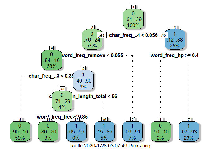
fancyRpartPlot(rpart_spam_pruning,      #fancy한 트리 생성
               cex = 1
               )
rpart_spam_predict<-predict(rpart_spam_pruning, test, type ='class')
confusionMatrix(rpart_spam_predict, test$class) #생성된 트리 모형의 평가(정확도, 민감도, 특이도 등)
## Confusion Matrix and Statistics
##
##           Reference
## Prediction   0   1
##          0 796 100
##          1  40 443
##
##                Accuracy : 0.8985
##                  95% CI : (0.8813, 0.9139)
##     No Information Rate : 0.6062
##     P-Value [Acc > NIR] : < 2.2e-16
##
##                   Kappa : 0.7832
##
##  Mcnemar's Test P-Value : 6.151e-07
##
##             Sensitivity : 0.9522
##             Specificity : 0.8158
##          Pos Pred Value : 0.8884
##          Neg Pred Value : 0.9172
##              Prevalence : 0.6062
##          Detection Rate : 0.5772
##    Detection Prevalence : 0.6497
##       Balanced Accuracy : 0.8840
##
##        'Positive' Class : 0
##
Random Forest
랜덤포레스트에 대한 설명은 링크를 참고해주세요.
data_rf <- randomForest(class ~ ., data = train)
data_rf
##
## Call:
##  randomForest(formula = class ~ ., data = train)
##                Type of random forest: classification
##                      Number of trees: 500
## No. of variables tried at each split: 7
##
##         OOB estimate of  error rate: 4.93%
## Confusion matrix:
##      0    1 class.error
## 0 1893   59  0.03022541
## 1  100 1170  0.07874016
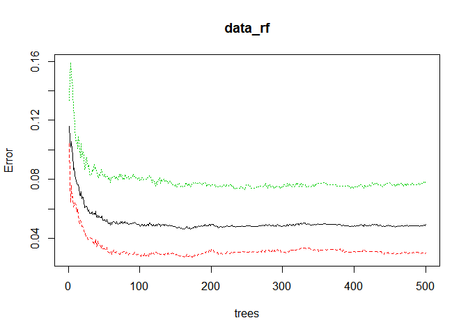
plot(data_rf) #나무의 갯수에 따른 오차율
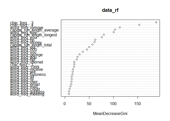
varImpPlot(data_rf) #변수 중요도(그래프에서 상단에 있을 경우 Label Data의 Class을 분류하는데 모델이 많이 활용하는 변수)
data_rf_predict <- predict(data_rf, test, type = "class")
confusionMatrix(data = data_rf_predict, reference=test$class) #생성된 RF모형의 평가(정확도, 민감도, 특이도 등)
## Confusion Matrix and Statistics
##
##           Reference
## Prediction   0   1
##          0 809  45
##          1  27 498
##
##                Accuracy : 0.9478
##                  95% CI : (0.9347, 0.9589)
##     No Information Rate : 0.6062
##     P-Value [Acc > NIR] : < 2e-16
##
##                   Kappa : 0.89
##
##  Mcnemar's Test P-Value : 0.04513
##
##             Sensitivity : 0.9677
##             Specificity : 0.9171
##          Pos Pred Value : 0.9473
##          Neg Pred Value : 0.9486
##              Prevalence : 0.6062
##          Detection Rate : 0.5867
##    Detection Prevalence : 0.6193
##       Balanced Accuracy : 0.9424
##
##        'Positive' Class : 0
##
모형 평가, 해석 및 선택
모형의 평가는 분류모형의 경우 혼동행렬(Confusion Matrix)에 기반하여 각 모형에 대한 정확도, 민감도, 특이도 등을 고려하여 종합적으로 평가하게 됩니다.
평가의 결과를 통해 두 모형 중 어떠한 모형으로 결정할 지 선택하게 됩니다.
시간이 너무 늦어 자세한 내용은 추후 업데이트하겠습니다.
오늘도 감사합니다.^^