rasch_4_1
Rasch_4_likert_1_NA
GitHub Documents
This is an R Markdown format used for publishing markdown documents to GitHub. When you click the Knit button all R code chunks are run and a markdown file (.md) suitable for publishing to GitHub is generated.
Including Code
You can include R code in the document as follows:
hls2 <- read.csv("data_pre.csv", header = T)
str(hls2)
## 'data.frame': 748 obs. of 45 variables:
## $ X : int 1 2 3 4 5 6 7 8 9 10 ...
## $ 癤풹chieve_1: int 0 0 0 2 1 1 3 3 1 3 ...
## $ achieve_2 : int 2 3 2 2 2 1 2 1 0 2 ...
## $ achieve_3 : int 1 2 4 2 0 3 4 0 2 1 ...
## $ achieve_4 : int 0 2 1 0 0 1 2 0 2 1 ...
## $ achieve_5 : int 0 0 1 1 0 1 3 0 1 2 ...
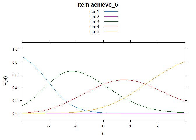
## $ achieve_6 : int 3 2 1 2 2 1 2 0 2 1 ...
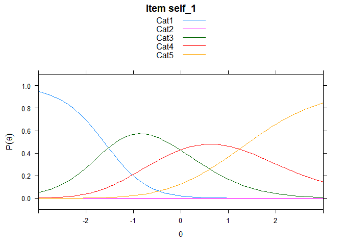
## $ self_1 : int 0 0 2 2 1 0 0 0 2 2 ...
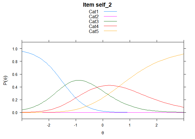
## $ self_2 : int 2 4 0 0 2 1 0 0 4 1 ...
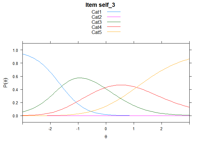
## $ self_3 : int 3 0 0 0 0 1 0 0 2 1 ...
## $ self_4 : int 2 4 3 0 2 2 4 0 2 1 ...
## $ self_5 : int 3 4 1 0 2 3 2 4 3 1 ...
## $ self_6 : int 2 3 0 2 0 0 0 0 1 0 ...
## $ self_7 : int 1 0 1 0 1 0 1 1 1 1 ...
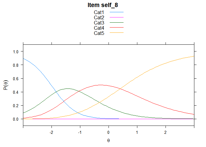
## $ self_8 : int 0 0 3 0 2 3 1 1 3 2 ...
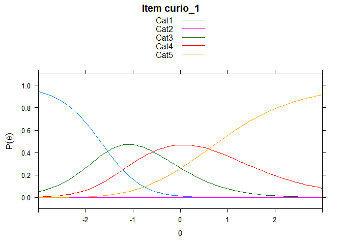
## $ curio_1 : int 0 0 1 0 0 0 0 0 4 0 ...
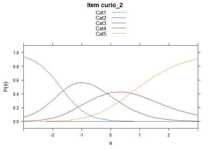
## $ curio_2 : int 0 0 1 0 0 1 0 0 0 0 ...
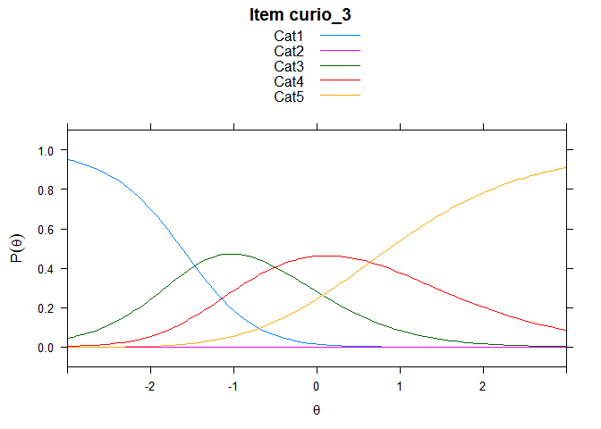
## $ curio_3 : int 1 0 3 0 0 2 0 4 4 0 ...
## $ curio_4 : int 1 0 1 0 0 0 0 4 0 1 ...
## $ curio_5 : int 1 0 0 4 1 1 0 1 0 1 ...
## $ curio_6 : int 0 0 0 4 2 2 0 0 0 1 ...
## $ curio_7 : int 1 0 0 0 0 0 0 0 0 1 ...
## $ curio_8 : int 2 0 1 2 1 3 0 4 0 4 ...
## $ curio_9 : int 1 0 0 2 0 0 0 0 0 1 ...
## $ curio_10 : int 0 0 0 4 2 0 0 4 0 0 ...
## $ curio_11 : int 0 0 0 0 0 0 0 0 0 1 ...
## $ info_1 : int 0 0 0 0 0 0 0 0 0 0 ...
## $ info_2 : int 0 0 1 0 1 0 0 1 0 0 ...
## $ info_3 : int 0 0 1 0 0 0 0 0 0 1 ...
## $ info_4 : int 0 0 0 0 0 0 2 0 1 2 ...
## $ info_5 : int 0 0 0 0 0 0 0 1 0 0 ...
## $ info_6 : int 2 0 1 0 2 0 2 0 0 3 ...
## $ inter_d_1 : int 1 0 2 4 4 4 2 4 2 2 ...
## $ inter_d_2 : int 1 4 0 2 4 3 2 4 2 1 ...
## $ inter_d_3 : int 2 4 1 2 4 3 2 4 2 2 ...
## $ inter_d_4 : int 1 0 2 1 4 1 4 4 2 0 ...
## $ inter_d_5 : int 1 4 2 2 0 1 2 0 2 0 ...
## $ inter_d_6 : int 0 0 4 2 0 3 2 0 2 2 ...
## $ inter_d_7 : int 0 0 3 0 0 1 0 1 2 1 ...
## $ inter_d_8 : int 0 0 0 3 0 2 0 0 2 1 ...
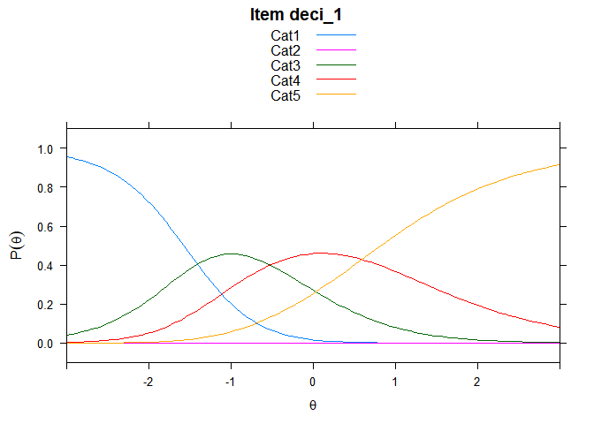
## $ deci_1 : int 3 4 1 1 4 1 4 4 2 3 ...
## $ deci_2 : int 3 0 2 2 4 4 2 0 2 3 ...
## $ deci_3 : int 2 4 4 2 4 4 4 3 2 3 ...
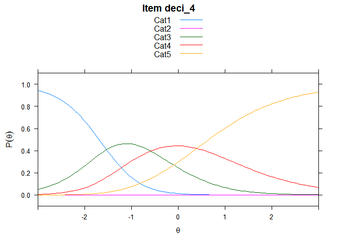
## $ deci_4 : int 2 2 0 2 2 2 4 4 2 4 ...
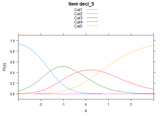
## $ deci_5 : int 2 2 4 4 3 2 4 3 2 4 ...
hls2[hls2 =="1"]<- NA

hls2 <- hls2[,2:45]
model fit
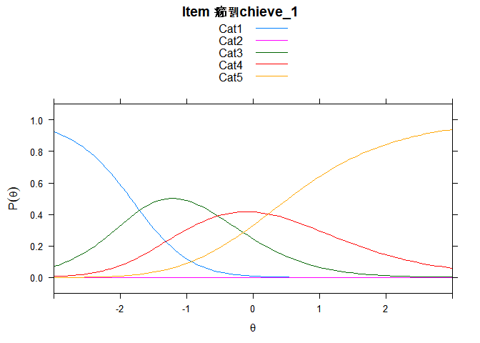
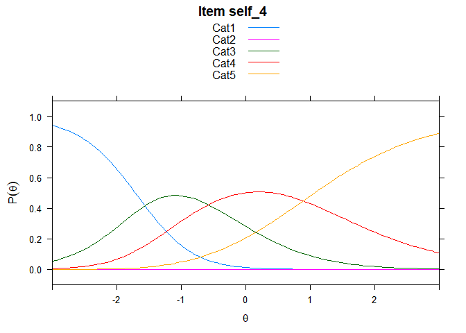
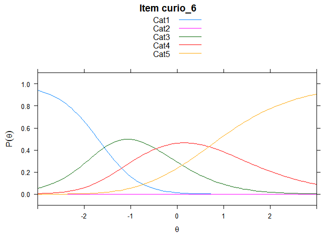
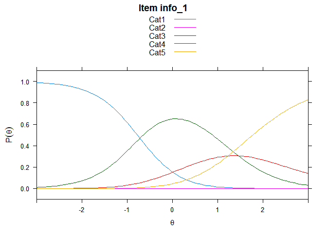
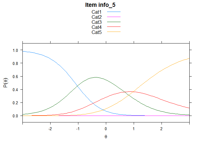
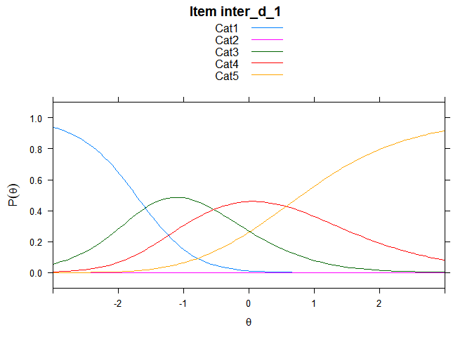
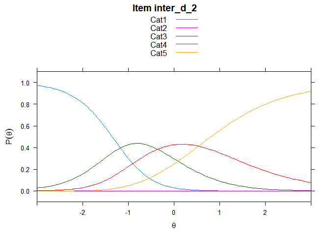
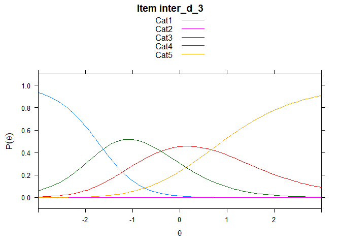
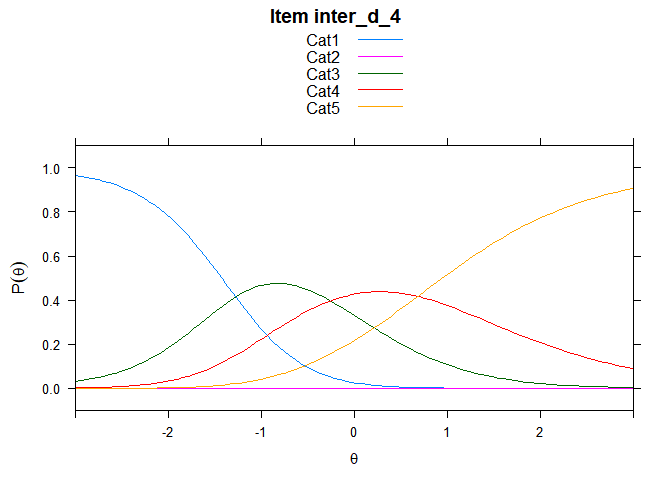
Including Plots
You can also embed plots, for example:
## Iteration in WLE/MLE estimation  1   | Maximal change  1.1858
## Iteration in WLE/MLE estimation  2   | Maximal change  0.2635
## Iteration in WLE/MLE estimation  3   | Maximal change  0.0123
## Iteration in WLE/MLE estimation  4   | Maximal change  1e-04
## Iteration in WLE/MLE estimation  5   | Maximal change  0
## ----
##  WLE Reliability= 0.912


## ....................................................
##  Plots exported in png format into folder:
##  C:/Users/Park Jung/Documents/rasch/teachnic_paper/rasch_4_1/rasch_4_1/Plots
Note that the echo = FALSE parameter was added to the code chunk to prevent printing of the R code that generated the plot.